An interest rate decision becomes meaningful to most people when it reaches their monthly budget. A household may have to set aside more for its home loan, a shopkeeper may find working capital more expensive, and a business owner may reconsider the timing of a new investment. These changes connect monetary policy to everyday choices about spending, saving and expansion.

On 7 October 2026, the Reserve Bank of India raised its policy repo rate by 25 basis points to 5.50%. The increase received unanimous support from the Monetary Policy Committee. [1] This paper describes how such a decision can pass through the economy and why its effects differ across households and businesses. Its central argument is that a rate hike can alter financial choices before it produces any visible relief in the prices of essential goods.

Monetary policy and the cost of borrowing

The repo rate is the rate on specified short-term lending by the RBI to banks against eligible securities. It influences the conditions under which banks obtain and price funds, although it is not the rate charged directly to every customer. A change of 25 basis points represents 0.25 percentage points. Its importance lies in how banks transmit that change into lending rates, deposit rates and the wider availability of credit.

The MPC adopted calibrated tightening, with two members preferring to retain a neutral stance. The resolution explains that a hike or a pause could follow under current conditions; another increase is not automatic. [1] For borrowers, this introduces uncertainty about future finance costs as well as the immediate question of when an existing loan will reset.

A floating-rate borrower experiences this transmission through the loan agreement. Where the rate is linked to the repo rate, a reset can increase the repayment amount, extend the remaining tenure, or affect both. The outcome depends on the contract and available repayment options. A fixed-rate contract normally retains its agreed rate for the fixed period, so households with similar outstanding debt may experience different effects.

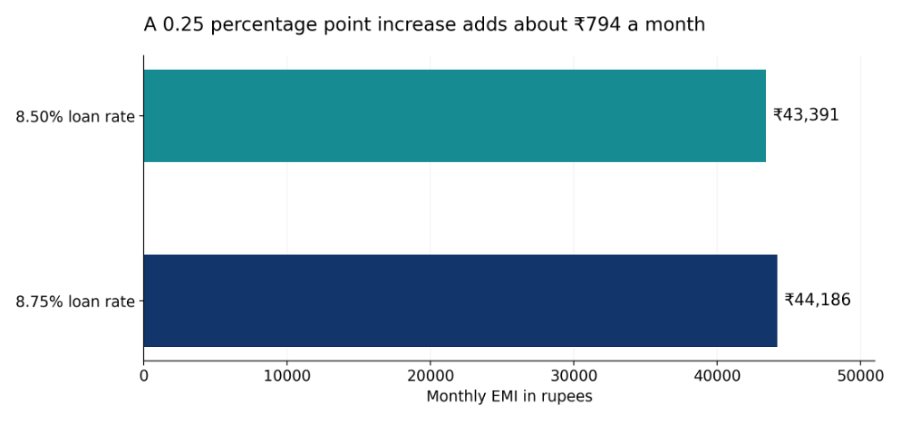
Illustration only: ₹50 lakh principal, 240 monthly payments, unchanged tenure and full 0.25 percentage point pass-through. Fees excluded. COSMINNOX calculation.

For the illustrative loan above, the EMI rises from ₹43,391.16 at 8.50% to ₹44,185.54 at 8.75%. The difference is ₹794.37 each month. If both rates remained unchanged for the entire 20 years, the total repayment difference would be about ₹190,650. This calculation describes a hypothetical loan; an existing borrower’s outcome depends on the outstanding balance and remaining tenure.

Debt repayment and everyday financial choices

A household budget is built around obligations that cannot all be adjusted with equal ease. Rent, school fees, food, electricity and loan repayments establish a substantial base of expenditure before a family considers travel, entertainment or a new purchase. When the interest component of debt rises, the household must accommodate that change somewhere within the same income. The adjustment may appear small when expressed as a percentage, but it becomes more visible when measured against the money left after essential bills.

Consider two families with similar incomes. One has a large floating-rate home loan, while the other rents and holds no debt. A rate reset may immediately change the first family’s financial commitments. The second may experience little direct repayment impact, although its members could still encounter changes in employment prospects, business income or returns on savings. This example illustrates why the policy rate does not create an identical household experience across the economy.

The remaining life of a loan also influences the adjustment. A borrower early in a long repayment schedule has more outstanding principal than one approaching the final instalments, assuming comparable original loans and repayment patterns. The effect of repricing must therefore be calculated from the current balance rather than simply applying the same increase to everyone who borrowed an identical amount years earlier. Changes in the EMI and tenure should be assessed together because a monthly payment can conceal a longer overall repayment commitment.

There is a behavioural dimension as well. Some families respond to financial uncertainty before their lender issues a revised schedule. They may postpone a large purchase or build a larger cash reserve because they expect future obligations to become harder to meet. Others continue spending because their incomes are stable or because the planned purchase is essential. Such choices are possible responses to uncertainty, not evidence that all consumers have already reduced expenditure after this particular announcement.

Savings decisions can also change. A family expecting higher deposit returns may find it more appealing to keep money aside, but that choice competes with debt repayment and immediate expenses. For a household carrying expensive debt, an increase in the income earned on a modest deposit may be smaller than the increase in borrowing costs. Whether the household gains or loses depends on both sides of its balance sheet, including the timing of rate resets.

Describing the household effect therefore requires more than the question of whether EMIs rise. The relevant picture includes debt exposure, income security, savings, essential expenditure and available repayment options. Monetary policy reaches daily life through the interaction of these circumstances. Its effect can be substantial for a household with limited spare income even when the announced rate change is modest.

Investment decisions and the household budget

The investment effects of higher rates develop through several channels. Banks may offer more attractive rates on new deposits, but the adjustment also depends on liquidity and competition for funds. Existing fixed deposits generally continue at their contracted rates until maturity. Savers therefore encounter the policy change through the terms available when they place or renew money, rather than through an immediate revision to every deposit.

Bonds respond differently. When market yields rise, the price of an existing fixed-coupon bond generally falls because its fixed payments become less attractive relative to newer alternatives. This matters particularly to an investor who sells before maturity. Higher yields on new bonds may improve prospective income, but maturity and credit quality remain relevant to the investment decision.

For equities, higher financing costs can reduce profits and make future earnings less valuable when discounted to the present. The consequences vary with a company’s debt, cash reserves and ability to maintain sales. Banks may benefit when loans reprice, while higher deposit costs or repayment stress can offset that advantage. These relationships describe economic mechanisms; they do not establish the direction of any individual share price.

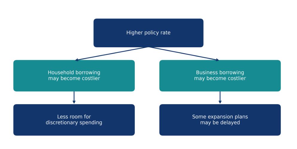
Conceptual channels rather than a measured forecast. Effects depend on contractual resets, income, liquidity and demand.

Household consumption is closely connected to these financial changes. When repayments absorb a larger share of an unchanged income, the money available for other purchases contracts. Families may postpone an appliance, reduce leisure spending or draw less on savings. The pressure is uneven: a household with substantial floating debt faces a different adjustment from one without loans. For small businesses, weaker discretionary demand can coincide with a higher interest bill on working capital, affecting both sales and the resources available for expansion.

Price pressures and the limits of a rate hike

The Governor’s October statement describes pressure from food and energy prices and deficient rainfall. It reports August CPI inflation at a rounded 4.8% and notes a broadening of underlying price pressures. [2] These conditions help explain why the relationship between higher rates and cheaper goods is indirect. The source of a price increase matters to the way policy can address it.

A higher borrowing rate cannot directly improve a harvest, repair a disrupted supply route or reduce the international cost of imported oil. Its influence works through spending decisions and expectations. When demand becomes less buoyant, firms may have less room to raise prices. When people expect inflation to moderate, the original supply shock may be less likely to spread into repeated increases across the economy. The RBI discusses this process in terms of second-round effects. [2]

Fuel, manufactured goods and gold also respond to different combinations of international prices, exchange rates, taxes and distribution costs. A movement in one component need not produce an equivalent movement in the final rupee price. This is why the effect of monetary policy should be understood as a gradual influence on inflation rather than an immediate reduction in the cost of every product.

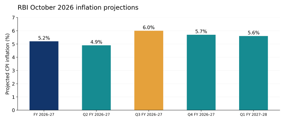
Source: RBI MPC resolution, 7 October 2026. Figures are forecasts. The full-year value is an annual average; the remaining values are quarterly averages. [1]

The October resolution projects CPI inflation at 5.2% for FY 2026–27 and real GDP growth at 7.1%. [1] These forecasts describe an expected path, not an assured outcome. A decline in inflation would ordinarily mean that prices were increasing more slowly; it would not necessarily restore the price level that households remember from an earlier period.

Small enterprises and the financing of daily operations

For a small enterprise, credit often finances the interval between paying for production and receiving payment from customers. A retailer buys stock before selling it, a manufacturer pays for materials before completing an order, and a service provider may pay salaries while waiting for an invoice to be settled. Working capital supports these gaps. When its interest cost rises, the business faces a higher expense even if output and sales remain unchanged.

A simple hypothetical example helps separate this effect from the home-loan illustration. If a business continuously uses ₹10 lakh of credit and its annual interest rate increases by 0.25 percentage points, the additional interest is approximately ₹2,500 over a year. The estimate assumes an unchanged balance for the whole year and excludes fees and compounding. Actual revolving-credit costs depend on daily utilisation, the reset date and the terms of the facility. The calculation describes an exposure, not a forecast for any particular firm.

The amount alone does not determine the pressure on the enterprise. A business with comfortable profit margins and prompt customer payments may absorb the increase. A firm operating on thin margins may find that a higher finance bill reduces the cash available to replenish stock or pay suppliers. If customers simultaneously become more cautious about spending, the enterprise can experience slower sales and more expensive credit at the same time.

The timing of receipts is particularly important. An order can be profitable on paper while still creating a cash shortage if payment arrives much later than expected. Higher interest increases the cost of financing that wait. For this reason, the effect of monetary policy on a business is connected to payment discipline, inventory management and the reliability of demand, as well as to the interest rate stated in its loan agreement.

Investment in new equipment adds another layer. The entrepreneur must weigh the expected improvement in capacity or productivity against the cost of financing and the likelihood of selling the additional output. A rate increase may shift the balance for a marginal project. A project supported by dependable orders or significant cost savings may still proceed. The decision is shaped by expected cash generation over time, rather than by the policy rate in isolation.

These differences matter when interpreting the position of micro, small and medium enterprises. The category includes businesses with widely varying debt, margins and customer relationships. Treating every enterprise as equally vulnerable would obscure that variation. A descriptive account instead follows the financing cycle within the business and considers where higher costs encounter an already narrow cash margin.

The wider implications for households and enterprises

COSMINNOX analysis: the policy tradeoff is most visible where essential expenses and debt repayments compete for the same income. Borrowers can feel a financial squeeze before slower inflation offers relief. For a small enterprise, the strain may emerge through the combined effect of financing costs, customer demand and the time taken to collect payments. A modest change in the policy rate can therefore have a larger practical significance for a borrower operating with little spare cash.

The adjustment is also shaped by choices within the household or firm. A borrower who accepts a longer tenure may preserve monthly spending capacity while paying interest for longer. A borrower who raises the EMI may avoid that extension but have less money available each month. Refinancing may change the calculation, although fees and the remaining repayment period affect whether it produces a real saving. The rate announcement alone is insufficient to establish the most suitable response.

For enterprises, the same principle applies to investment. A project that appeared viable under cheaper credit may require a fresh assessment of expected demand and cash flow. Yet higher rates do not make all expansion uneconomic. Businesses with reliable orders, adequate reserves and limited debt may continue to invest, while firms dependent on short-term borrowing may postpone expenditure. The economic response emerges from these differing positions rather than from a uniform reaction across all sectors.

Monetary policy also operates alongside supply conditions. Improvements in food storage, transport and energy reliability can address constraints that interest rates cannot remove. Clear communication about loan resets can help borrowers understand the change in their obligations. These are COSMINNOX recommendations, distinct from the RBI’s announced measures, and reflect the need to consider both financial transmission and the sources of price pressure.

The timing of monetary policy transmission

The interval between a policy announcement and its wider economic effect is central to understanding a rate hike. Financial markets can respond quickly to expectations, while loan contracts reprice according to their reset schedules. Spending decisions then develop as borrowers experience the revised cost or anticipate it. The influence on inflation depends on how those changes interact with production, supplies and price-setting behaviour. There is no single date on which the entire economy moves to the new conditions.

This sequence makes immediate judgements difficult. A movement in a share index on the day of the announcement may reflect expectations about interest rates alongside earnings news, global markets or commodity prices. An unchanged EMI during the following month may simply reflect a later contractual reset. Neither observation, by itself, establishes the full effect of the policy decision. A descriptive assessment must keep the financial response and the real-economy response in view without assuming that they unfold simultaneously.

The same care is needed when interpreting prices. Inflation is the rate of change in a price index, while the price level is the accumulated cost of the basket. If inflation slows but remains positive, that basket still becomes more expensive, although at a reduced pace. A household may consequently continue to feel pressure even when the statistical measure improves. Its own purchases may also differ from the representative basket, particularly where food or other essentials absorb a large share of spending.

Supply developments can strengthen or weaken the transmission. Better availability of a food item can ease its price independently of the interest rate, while a new supply disruption can raise prices despite more restrained demand. Exchange-rate movements and international commodity costs can further complicate the result. It would therefore be misleading to attribute every subsequent price movement entirely to the rate hike.

The quality of the assessment depends on observing several developments together: changes in lending conditions, the evolution of household demand, the cost of business finance and the breadth of price pressures. Forecasts provide a reference for that observation, but they must remain distinct from realised outcomes. This approach allows the paper to explain the policy’s potential significance without presenting its eventual effects as already settled.

Conclusion

The October repo rate increase connects a national policy decision to household repayments, saving opportunities and business finance. Its effects are likely to appear at different times because contracts, balance sheets and spending needs differ. Understanding that variation is essential to interpreting the decision: higher borrowing costs can influence demand and inflation, while essential prices continue to respond to supply, currencies and domestic costs. The outcome will depend on how these forces develop together.

Sources and references

Tier 1 = primary government or regulator document. Tier 2 = credible secondary reporting. Tier 3 = attributed opinion or self-reported claim.